Using simulation to make hard math easy: How to Catch a T-Shirt at a Music Festival

I decided to take a stab at this week’s Riddler from FiveThirtyEight.com. It’s a weekly puzzle series that focuses on math, logic, and probability. The series is a great opportunity to stretch your brain and sometimes your coding skills. I used a Python simulation to solve this week’s challenge.

The Challenge

Read the original challenge here.

During a break at a music festival, the crew is launching T-shirts into the audience using a T-shirt cannon. And you’re in luck — your seat happens to be in the line of flight for one of the T-shirts! In other words, if the cannon is strong enough and the shirt is launched at the right angle, it will land in your arms.

The rows of seats in the audience are all on the same level (i.e., there is no incline), they are numbered 1, 2, 3, etc., and the T-shirts are being launched from directly in front of Row 1. Assume also that there is no air resistance (yes, I know, that’s a big assumption). You also happen to know quite a bit about the particular model of T-shirt cannon being used — with no air resistance, it can launch T-shirts to the very back of Row 100 in the audience, but no farther.

The crew member aiming in your direction is still figuring out the angle for the launch, which you figure will be a random angle between zero degrees (straight at the unfortunate person seated in Row 1) and 90 degrees (straight up). Which row should you be sitting in to maximize your chances of nabbing the T-shirt?

The Approach

My approach to this problem was to solve it with a simulation rather than solve it analytically. More about this decision later. I set up a simulation that will launch a T-shirt at a constant velocity (according to the specs of our cannon) and at a random angle. If I run this simulation enough times and record the row where the T-shirt lands after each launch, the simulation should converge on a solution. The row where the T-shirt landed most often will be the row with the best odds of catching a T-shirt. But not necessarily the row with the best view of the show.

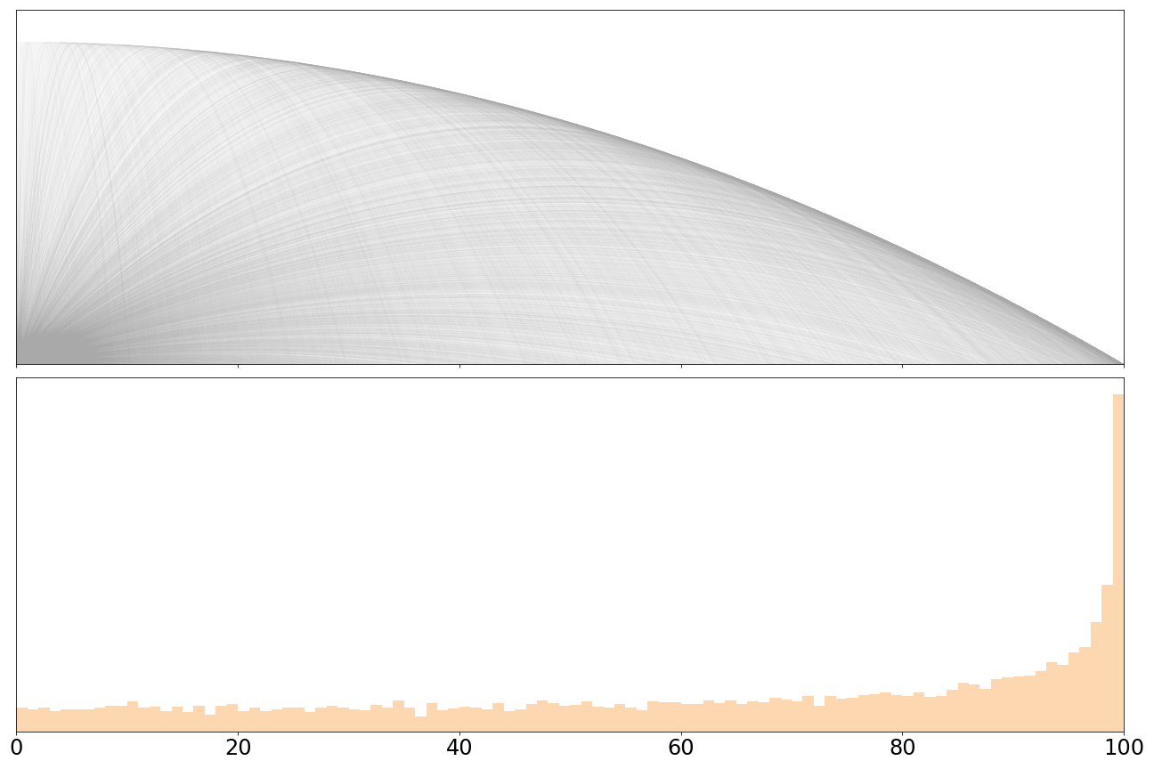
Here’s what the model looks like while running through the first 100 simulations. The histogram in the lower panel is split into 100 bins. The bin that’s the tallest represents the row with the best chance of catching the T-shirt.

The Solution

Here’s what the model looks like after running 10,000 times. It shows that sitting in the back row will give you the best chance at catching the shirt.

How I did it

To create the model, I started with the kinematic equations from Physics 101 that describe projectile motion. You can describe the trajectory of the T-shirt if you know the initial velocity and the launch angle.

First you need to break down the velocity vector into its x- and y-components:

\[V_{y0} = V_0 * sin(\theta)\] \[V_{x0} = V_0 * cos(\theta)\]

Then, you solve the location equations.

\[x = x_0 + V_{x0} t\] \[y = y_0 + V_{y0}t + \frac{1}{2}at^2\]

In the case of our T-shirt cannon, I want to solve these equations for the initial velocity of the cannon. We know that the initial and final Y position are the same because the floor is not sloped, a is the acceleration due to gravity, 9.81 m/s^2, and I will assume that the final X position is 100m. This assumes the seats are spaced 1 meter apart. A little long for a festival, but it will make the calculations and visualizations simpler.

We are given the maximum distance the cannon can shoot as 100m. In order to reach its maximum range, the cannon must be fired at 45 degrees. A 45 degree launch angle will always result in the maximum horizontal distance traveled when air resistance is ignored. For an explanation of why this is the case, look here.

With all of this information, we can solve the above equations to determine that the initial total velocity of the cannon is 31.32m/s.

(It isn’t totally necessary to calculate the cannon velocity. We could alternatively pick an arbitrary velocity and divide the resulting distance into 100 rows. That’s why it’s fine to assume the seats are spaced 1m apart.)

Now, let’s define a class in Python to describe the T-shirt. It will take the launch speed and launch angle as parameters, and it will have methods to calculate the time the T-shirt is in the air, the total horizontal distance the T-shirt travels, and the trajectory in the x and y directions.

import numpy as np

class TShirt:

  def __init__(self, launch_speed, launch_angle):
    self.Vo = launch_speed
    self.Vox = self.Vo * np.cos(launch_angle) # initial x velocity
    self.Voy = self.Vo * np.sin(launch_angle) # initial y velocity

    self.a = -9.81 # acceleration due to gravity


  def air_time(self):
    # solve the quadratic y_f = y_0 + (V_y0 * t) + (1/2 * a * t^2) 
    # for t where y_0 == y_f
    return np.roots((1/2 * self.a, self.Voy, 0))[0] 


  def final_x(self):
    return self.Vox * self.air_time()


  def x_trajectory(self):
    t = np.linspace(0, 10, 500)
    x = 0 + self.Vox * t
    return x
  

  def y_trajectory(self):
    t = np.linspace(0, 10, 500)
    y = 0 + self.Voy * t + 1/2 * self.a * t ** 2  
    return y

To see how this works, we can define a T-shirt that is launched out of our cannon at 45 degrees (pi/4 radians). We can execute the air_time and final_x methods on the tshirt to calculate those values.

>>> tshirt = TShirt(31.32, np.pi/4)
>>> tshirt.air_time()
4.51
>>>tshirt.final_x()
99.99

Now that we have the class defined, we can create a large number of instances that are launched at random angles between 0 and 90 degrees. Running the code below will calculate the maximum X position and trajectories for 10,000 T-Shirt cannon launches.

nruns = 10_000
V = 31.32

# initialize arrays to fill with values
max_xs = np.ndarray((nruns,))
x_trajectories = np.ndarray((nruns, 500))
y_trajectories = np.ndarray((nruns, 500))

# generate the random angles
thetas = np.random.random((nruns)) * np.pi / 2

for i, theta in enumerate(thetas):
   tshirt = TShirt(V, theta)
   max_xs[i] = tshirt.final_x()
   x_trajectories[i,:] = tshirt.x_trajectory()
   y_trajectories[i, :] = tshirt.y_trajectory()

With the simulations done, we can make a plot to inspect the results.

import seaborn as sns
import matplotlib.pyplot as plt

fig, (ax1, ax2) = plt.subplots(figsize=(18, 12), nrows=2, ncols=1, sharex=True)
ax1.plot(x_trajectories.T, y_trajectories.T, color='gray', alpha=.01)
ax1.set_xlim(0, 100)
ax1.set_yticks([])
ax1.set_ylim(0, 55)

ax2 = sns.distplot(max_xs, kde=False, bins=100)
ax2.set_yticks([])
ax2.tick_params(axis='x', labelsize=24)

fig.tight_layout()

The Wrap Up

With a bit more algebra and some calculus, this problem could have been solved analytically, meaning with pure math and no need for code. I think it’s a great example of how knowing how to approach problems from a coding perspective can make some math problems simpler.

I’m inspired by one of my favorite PyCon talks by Jake Vanderplas, Statistics for Hackers. The point of the talk is that statistics is hard, but by applying some programming skill, you can make it easier. If you can write a for-loop, he says, you can do statistics. I took the same approach here. If you can write a for-loop, you can catch a free music festival T-shirt.